Hertz Contact Stress in Deep Groove Ball Bearings — Analytical Pipeline

Quick Example

What this tool does, in 30 seconds. Given a bearing designation and a radial load, the pipeline computes the maximum subsurface shear stress and tells you how close you are to the material limit.

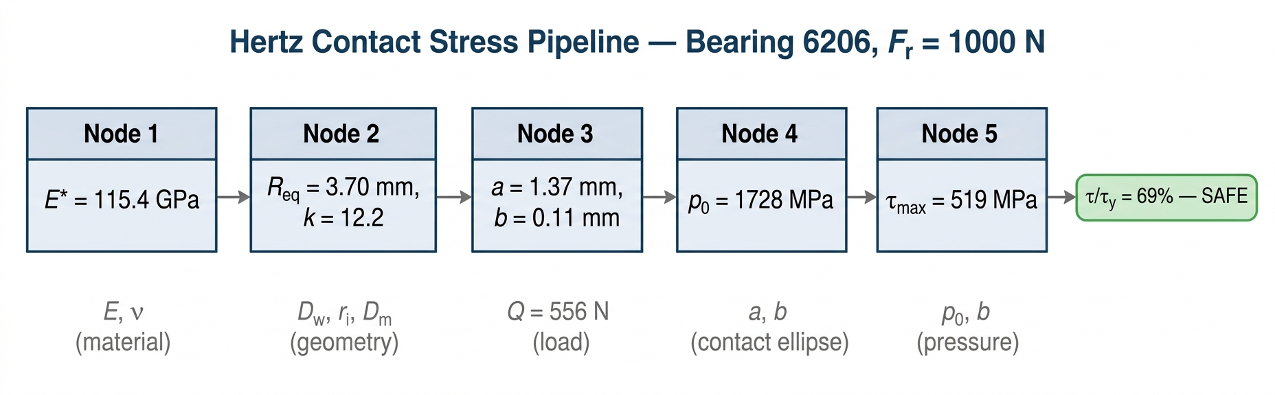
Input: Bearing 6206, radial load 1000 N, AISI 52100 steel ( \(E = 210\) GPa, \(\nu = 0.3\) ). Ball Ø 9.525 mm, inner groove radius 4.89 mm, pitch diameter 46.0 mm, 9 balls, \(\alpha = 0°\) .

\[ \boxed{\tau_{\max} = 519 \text{ MPa} \quad \text{at} \quad z_{cr} = 88 \;\mu\text{m below the surface}} \]

The maximum subsurface shear stress is 69 % of the shear yield strength of hardened AISI 52100 ( \(\tau_y \approx 750\) MPa, Tresca). Margin to yield: 31 %. Infinite fatigue life expected at this load level.

Check	Value	Limit	Status
\(\tau_{\max} / \tau_y\)	69 %	100 %	Safe — 31 % margin
\(\tau_{\max} / \tau_{fatigue}\)	76 %	100 %	Below fatigue limit
\(F_r / C_0\)	8.9 %	100 %	Light load

Node	Quantity	Value	Unit
1	Reduced elastic modulus \(E^*\)	115.4	GPa
2	Equivalent radius \(R_{eq}\)	3.700	mm
2b	Ellipticity \(k = a/b\)	12.19	—
3	Contact semi-axes \(a \times b\)	1.368 × 0.112	mm
4	Max contact pressure \(p_0\)	1728	MPa
5	Max shear stress \(\tau_{\max}\)	519	MPa
5	Critical depth \(z_{cr}\)	88	μm

📓 Open in Google Colab to run the calculation with your own bearing data.

Pipeline Overview

The pipeline takes bearing geometry, material properties, and radial load as input. It outputs the maximum subsurface shear stress \(\tau_{\max}\) and its depth \(z_{cr}\) , which govern fatigue initiation at the ball–raceway contact.

5-node Hertz contact stress pipeline from bearing geometry to subsurface shear stress

The pipeline is linear and non-iterative. The only potentially iterative step (elliptic integrals in Node 2b) is handled by the Hamrock-Brewe closed-form approximation.

Node 1 — Reduced Elastic Modulus \(E^*\)

Purpose: combine the elastic properties of ball and raceway into a single equivalent modulus.

Symbol	Description	Unit
\(E_1\)	Young’s modulus, ball	Pa
\(\nu_1\)	Poisson’s ratio, ball	—
\(E_2\)	Young’s modulus, raceway	Pa
\(\nu_2\)	Poisson’s ratio, raceway	—

\[ \frac{1}{E^*} = \frac{1 - \nu_1^2}{E_1} + \frac{1 - \nu_2^2}{E_2} \]

Harris convention (used in Nodes 3–4):

\[E' = 2 \, E^*\]

Output	Description	Unit
\(E^*\)	Reduced elastic modulus	Pa
\(E'\)	Harris reduced modulus	Pa

Node 2 — Curvatures and Equivalent Radius

Purpose: compute the four principal curvatures at the ball–inner-race contact and combine them into an equivalent radius \(R_{eq}\) and an ellipticity parameter.

Input	Description	Unit
\(D_w\)	Ball diameter	m
\(r_i\)	Inner race groove radius	m
\(D_m\)	Pitch (mean) diameter	m
\(\alpha\)	Contact angle	rad

The two principal planes at the contact point are:

Plane I (rolling direction): circumferential plane through ball centre.
Plane II (transverse direction): axial cross-section through ball centre.

Ball (sphere):

\[\rho_{1x} = \rho_{1y} = \frac{2}{D_w}\]

Inner raceway:

\[ \rho_{2x} = \frac{2}{D_m - D_w \cos\alpha} \qquad\text{(convex, rolling)} \]

\[ \rho_{2y} = -\frac{1}{r_i} \qquad\text{(concave, transverse)} \]

The negative sign indicates that the groove is concave — it wraps around the ball.

Curvature sums:

\[ \frac{1}{R_x} = \rho_{1x} + \rho_{2x} \qquad \frac{1}{R_y} = \rho_{1y} + \rho_{2y} \]

\[ \Sigma\rho = \frac{1}{R_x} + \frac{1}{R_y} \qquad R_{eq} = \frac{1}{\Sigma\rho} \]

Ellipticity (Hamrock-Brewe 1983)

The ratio \(R_y/R_x\) determines the shape of the contact ellipse. The Hamrock-Brewe closed-form approximation replaces iterative evaluation of complete elliptic integrals:

\[ k = 1.0339\left(\frac{R_y}{R_x}\right)^{0.6360} \]

\[ \mathcal{E} = 1.0003 + \frac{0.5968}{R_y/R_x} \qquad \mathcal{F} = 1.5277 + 0.6023 \, \ln\!\left(\frac{R_y}{R_x}\right) \]

where \(k = a/b\) is the ellipticity ratio, \(\mathcal{E}\) the complete elliptic integral of the second kind, \(\mathcal{F}\) the first kind. Accurate to < 1 % for \(R_y/R_x > 1\) .

Why Hamrock-Brewe? Exact evaluation requires iterative root-finding (the argument depends on \(k\) , which depends on the integrals). The Hamrock-Brewe formulas break this circularity, keeping the pipeline non-iterative and scipy-free.

Output	Description	Unit
\(R_{eq}\)	Equivalent radius	m
\(k\)	Ellipticity ratio \(a/b\)	—
\(\mathcal{E}\)	Elliptic integral, 2nd kind	—
\(\mathcal{F}\)	Elliptic integral, 1st kind	—

Node 3 — Contact Ellipse Semi-Axes

Purpose: compute the dimensions of the elliptical contact patch.

The load on the most-loaded ball follows the Stribeck equation (zero clearance):

\[ Q_{\max} = \frac{5 \, F_r}{Z \, \cos\alpha} \]

Contact semi-axes (Hamrock-Dowson):

\[ b = \left(\frac{6 \, \mathcal{E} \, Q \, R_{eq}}{\pi \, k \, E'}\right)^{1/3} \qquad a = k \, b \]

where \(a\) is the major semi-axis (transverse) and \(b\) the minor (rolling direction).

Output	Description	Unit
\(Q_{\max}\)	Load on most-loaded ball	N
\(a\)	Major semi-axis	m
\(b\)	Minor semi-axis	m

Node 4 — Maximum Contact Pressure

Purpose: peak Hertzian pressure at the centre of the contact ellipse.

\[ p(x, y) = p_0 \sqrt{1 - \frac{x^2}{a^2} - \frac{y^2}{b^2}} \]

\[ p_0 = \frac{3 \, Q}{2 \, \pi \, a \, b} \]

Output	Description	Unit
\(p_0\)	Maximum contact pressure	Pa

Node 5 — Maximum Shear Stress and Critical Depth

Purpose: maximum subsurface shear stress (Tresca) and the depth where fatigue cracks initiate.

For \(k \gg 1\) (highly elliptical, typical of ball bearings), the stress field approximates 2D plane-strain Hertz contact in the \(b\) -direction (< 1 % error for \(k > 5\) ).

Subsurface stresses along the \(z\) -axis:

\[ \frac{\sigma_x}{p_0} = -\left[\frac{1 + 2\zeta^2}{\sqrt{1+\zeta^2}} - 2\zeta\right] \qquad \frac{\sigma_z}{p_0} = -\frac{1}{\sqrt{1+\zeta^2}} \qquad \zeta = z/b \]

\[ \sigma_y = \nu \, (\sigma_x + \sigma_z) \qquad \tau = \frac{\sigma_x - \sigma_z}{2} \]

Analytical maximum:

\[ \tau_{\max} = 0.300 \, p_0 \qquad\text{at}\qquad \zeta_{cr} = 0.786 \qquad\Rightarrow\qquad z_{cr} = 0.786 \, b \]

Output	Description	Unit
\(\tau_{\max}\)	Maximum subsurface shear stress	Pa
\(z_{cr}\)	Critical depth below surface	m

Numerical Verification — Bearing 6206

Input Data

Parameter	Symbol	Value	Unit	Source
Bore diameter	\(d\)	30	mm	Catalog
Outer diameter	\(D\)	62	mm	Catalog
Ball diameter	\(D_w\)	9.525	mm	Catalog
Number of balls	\(Z\)	9	—	Catalog
Inner groove radius	\(r_i\)	4.89	mm	Catalog ( \(f_i = 0.513\) )
Pitch diameter	\(D_m\)	46.0	mm	\((d+D)/2\)
Contact angle	\(\alpha\)	0	°	Deep groove, radial
Young’s modulus	\(E\)	210	GPa	AISI 52100
Poisson’s ratio	\(\nu\)	0.3	—	AISI 52100
Radial load	\(F_r\)	1000	N	Test condition
Static load rating	\(C_0\)	11.2	kN	SKF catalog

Node-by-Node Computation

Node 1:

\[ \frac{1}{E^*} = 2 \times \frac{1 - 0.3^2}{210\,000} = 8.667 \times 10^{-6} \text{ MPa}^{-1} \qquad\Rightarrow\qquad E^* = 115.4 \text{ GPa}, \quad E' = 230.8 \text{ GPa} \]

Node 2: Ball radius \(r_{ball} = 4.7625\) mm. Curvatures: \(\rho_{1x} = \rho_{1y} = 209.97\) m \(^{-1}\) .

Inner race: \(R_{2x} = (46.0 - 9.525)/2 = 18.238\) mm → \(\rho_{2x} = 54.83\) m \(^{-1}\) . \(\rho_{2y} = -1/4.89 = -204.50\) m \(^{-1}\) (concave groove).

\(1/R_x = 264.81\) m \(^{-1}\) → \(R_x = 3.776\) mm. \(1/R_y = 5.475\) m \(^{-1}\) → \(R_y = 182.7\) mm. \(\Sigma\rho = 270.3\) m \(^{-1}\) , \(R_{eq} = 3.700\) mm, \(R_y/R_x = 48.37\) .

Hamrock-Brewe: \(k = 12.19\) , \(\mathcal{E} = 1.013\) , \(\mathcal{F} = 3.864\) .

Node 3: \(Q_{\max} = 5 \times 1000 / 9 = 555.6\) N.

\[ b = \left(\frac{6 \times 1.013 \times 555.6 \times 3.700 \times 10^{-3}} {\pi \times 12.19 \times 230\,769}\right)^{1/3} = 0.1122 \text{ mm} \]

\(a = 12.19 \times 0.1122 = 1.368\) mm. Contact area: \(A = 0.482\) mm².

Node 4:

\[ p_0 = \frac{3 \times 555.6}{2\pi \times 1.368 \times 0.112} = 1728 \text{ MPa} \]

Cross-check: sphere-on-flat gives \(p_0 = 3981\) MPa — groove conformity reduces pressure by 2.3×.

Node 5: \(\tau_{\max} = 0.300 \times 1728 = 518.5\) MPa at \(z_{cr} = 0.786 \times 0.112 = 88\) μm. Numerical scan confirms \(\tau_{\max} = 518.9\) MPa at \(\zeta = 0.786\) (deviation < 0.1 %).

Verification Summary

Quantity	Computed	Unit	Check
\(E^*\)	115.4	GPa	Matches \(E/(2(1-\nu^2))\) for same-steel contact
\(R_{eq}\)	3.700	mm	\(R_x \ll R_y\) confirms high ellipticity
\(k\)	12.19	—	Typical range 8–15 for DGBB
\(a\)	1.368	mm	Contact patch ≈ grain of rice
\(b\)	0.112	mm	\(a/b = k\) ✓
\(p_0\)	1728	MPa	Well below 4600 MPa ( \(C_0\) limit) at 9 % \(C_0\)
\(\tau_{\max}\)	519	MPa	69 % of \(\tau_y\) — safe, consistent with light load
\(z_{cr}\)	88	μm	≈ \(0.8 b\) , matches 2D Hertz theory

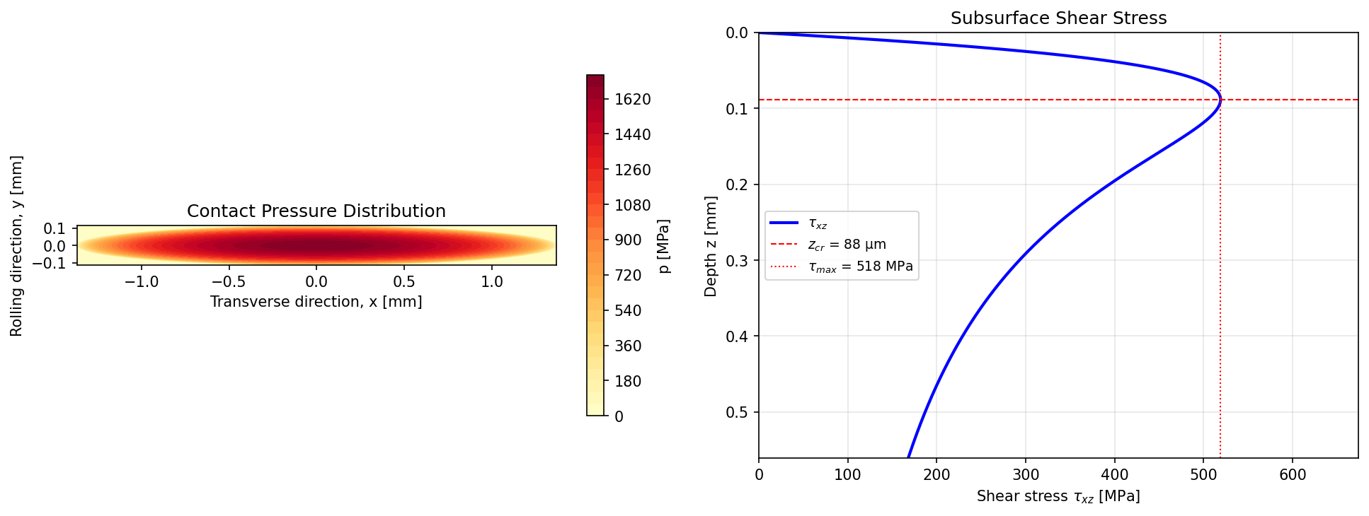
Graphical Results

Figure 1 — Left: Hertzian pressure distribution on the contact ellipse (1728 MPa peak, ellipse ≈ 2.7 × 0.22 mm). Right: subsurface shear stress profile showing the maximum at \(z_{cr} = 88\) μm.

Hertz contact pressure distribution and subsurface shear stress — bearing 6206 at 1000 N radial load

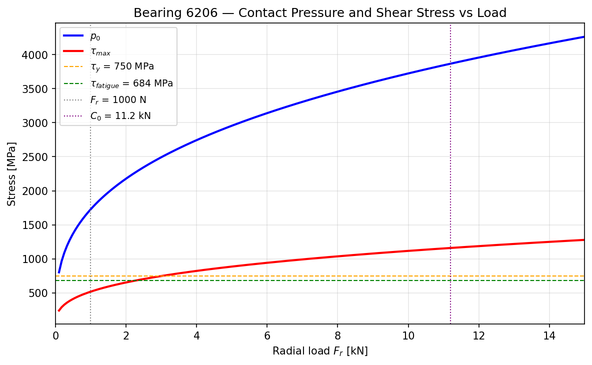
Figure 2 — Maximum contact pressure \(p_0\) and subsurface shear stress \(\tau_{\max}\) vs radial load. Horizontal lines: shear yield and fatigue limits. Vertical lines: current load (1000 N) and static rating ( \(C_0 = 11.2\) kN).

Parametric plot of maximum contact pressure vs radial load for bearing 6206

How to Use the Notebook

Requirements

Only numpy and matplotlib — both pre-installed in Google Colab.

Running

Open hertz_contact_stress_pipeline.ipynb directly in Colab.
Edit the Input Parameters cell with your bearing data.
Run all cells (Runtime → Run all).

Adapting to Other Bearings

Look up \(D_w\) , \(Z\) , \(d\) , \(D\) from manufacturer catalog.
Compute \(r_i = f_i \times D_w\) (typical \(f_i = 0.515\) –\(0.52\) ; use 0.52 if unknown).
Update E1, E2, nu1, nu2 if material differs from steel.
Set alpha > 0 for angular contact bearings.

Limitations

Inner race contact only. Outer race (less critical for DGBB) not computed.
Zero clearance assumed. Stribeck factor assumes no radial clearance or preload.
Plane-strain approximation for \(\tau_{\max}\) . Valid for \(k > 5\) .
Static/quasi-static only. No centrifugal or gyroscopic effects.

References

Anoopnath, P. R., Suresh Babu, V., & Vishwanath, A. K. (2018). Hertz Contact Stress of Deep Groove Ball Bearing. Materials Today: Proceedings, 5(1), 3283–3288.
Hamrock, B. J. & Brewe, D. E. (1983). Simplified equation for elliptical-contact deformation between two elastic solids. ASME J. Lub. Tech., 105(2), 171–177.
Harris, T. A. & Kotzalas, M. N. (2006). Rolling Bearing Analysis, 5th ed. CRC Press.
Johnson, K. L. (1985). Contact Mechanics. Cambridge University Press, §4.2.
Budynas, R. G. & Nisbett, J. K. (2020). Shigley’s Mechanical Engineering Design, 11th ed. McGraw-Hill, §3.19.
SKF Group. Product data: 6206 Deep Groove Ball Bearing.

Quick Example#

Pipeline Overview#

Node 1 — Reduced Elastic Modulus \(E^*\)

Node 2 — Curvatures and Equivalent Radius#

Ellipticity (Hamrock-Brewe 1983)#

Node 3 — Contact Ellipse Semi-Axes#

Node 4 — Maximum Contact Pressure#

Node 5 — Maximum Shear Stress and Critical Depth#

Numerical Verification — Bearing 6206#

Input Data#

Node-by-Node Computation#

Verification Summary#

Graphical Results#

How to Use the Notebook#

Requirements#

Running#

Adapting to Other Bearings#

Limitations#

References#