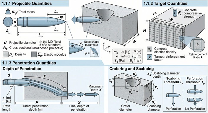
Over six decades of ballistic testing have produced dozens of empirical formulae for concrete penetration — NDRC, Barr (UKAEA), ACE. All three share the same structural defects: unit-dependent coefficients that break when switching from SI to imperial, nose shape parameters assigned as discrete lookup values rather than computed from geometry, and calibration ranges limited to shallow impacts (\(0.6 < X/d < 2.0\) ) that collapse at deep penetration (\(X/d > 5\) ) with errors exceeding 20%.
Li & Chen (2003) resolved these defects by building on two independent pillars. The Buckingham Pi theorem reduces the 10 physical variables of the problem to three dimensionless groups: the impact factor \(I^*\) , the mass ratio \(\lambda\) , and the nose factor \(N^*\) . Dynamic cavity expansion theory (Forrestal & Luk 1988) then provides the axial force law — static confinement resistance plus inertial resistance — and introduces the empirical parameter \(S\) that bridges uniaxial compressive strength to effective confined resistance. Combining the two theories recombines the three Pi groups into two operational numbers, \(I\) and \(N\) , which govern the result entirely.
The outcome is two closed-form formulae — Eq. (15a) for shallow penetration, Eq. (15b) for deep — validated against approximately 130 data points covering \(X/d\) from 0.07 to 92.8.
Quick Example
4340-steel ogive projectile, CRH = 2, impacting 35 MPa concrete at 277 m/s. Data: Forrestal et al. (1994), Table 3, shot 14.
| Input | Value |
|---|---|
| Mass \(M\) | 0.906 kg |
| Diameter \(d\) | 26.9 mm |
| Nose type | Ogive, CRH \(\psi = 2\) |
| Impact velocity \(V_0\) | 277 m/s |
| Compressive strength \(f_c\) | 35.2 MPa |
| Concrete density \(\rho_c\) | 2370 kg/m³ |
Penetration depth: \(X = 167\,\text{mm}\) (\(X/d = 6.21\) , deep regime) Test measurement: 173 mm. Model error: 3.4%. NDRC prediction: 137 mm. NDRC error: 20.5%.
The 26.9 mm ogive projectile at 277 m/s penetrates 167 mm into 35 MPa concrete — about 6.2 calibers. At this velocity the static resistance term accounts for 94% of the retarding force; the dynamic inertia term contributes only 6%. NDRC, calibrated on shallow impacts, underestimates by a factor that grows with penetration depth.
Pipeline summary:
| Node | Operation | Key output |
|---|---|---|
| 0 | Validity check | ✅ \(V_0 = 277\) m/s \(< 800\) m/s, rigid projectile |
| 1 | Nose geometry | \(N^* = 0.156\) , \(k = 2.030\) |
| 2 | Target resistance | \(S = 12\) (paper) |
| 3 | Dimensionless numbers | \(I = 8.455\) , \(N = 125.9\) |
| 4 | Regime | \(I = 8.455 > \pi k/4 = 1.571\) → deep penetration |
| 5b | Eq. (15b) | \(X/d = 6.21\) |
| 6 | Dimensional output | \(X = 167\,\text{mm}\) |
Pipeline Overview
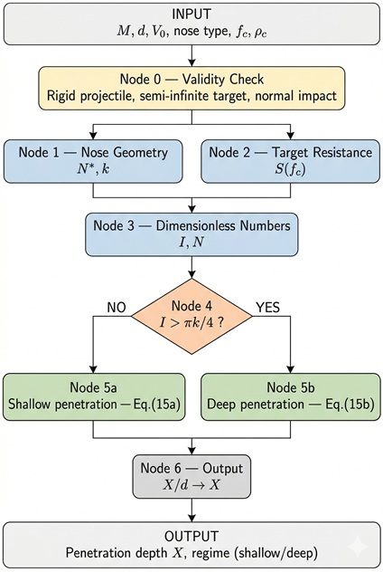
The pipeline is sequential with one bifurcation. Nodes 0–3 are always executed. Node 4 selects the depth formula based on whether \(I\) exceeds the crater threshold \(\pi k/4\) . Node 5a (shallow) or 5b (deep) computes the dimensionless depth; Node 6 converts to metres or millimetres.
📄 Download: The A4 Ballistic Pipeline — slide deck (PDF) - A visual representation of the calculation
📄Download The Theory Behind the Calculation (PDF) — A visual walkthrough of the physics: from Buckingham Pi to cavity expansion to the final dimensionless equations.
Node 0 — Validity Pre-Check
Purpose. Verify that the model assumptions hold before computing. If a condition is violated, the pipeline emits a warning but does not block execution — the engineering judgement remains with the user.
| Input | Symbol | Unit |
|---|---|---|
| Impact velocity | \(V_0\) | m/s |
| Shank diameter | \(d\) | m |
| Aggregate size (optional) | \(a\) | m |
| Condition | Criterion | Reference |
|---|---|---|
| Rigid (non-deformable) projectile | \(V_0 \lesssim 800\,\text{m/s}\) for hardened steel | Paper §2.1 |
| Semi-infinite target | thickness \(\geq 3X\) — verify after calculation | Model assumption |
| Normal incidence | impact angle = 90° | Model assumption |
| Aggregate small vs. diameter | \(d/a \gg 1\) (ideally \(> 5\) ) | Paper §2.1 |
| Light or no reinforcement | \(< 1.5\%\) per direction | Paper §2.1 |
| Output | Symbol |
|---|---|
| Status (pass / warning list) | — |
Node 1 — Nose Geometry
Purpose. Compute the nose shape factor \(N^*\) and the dimensionless crater depth \(k\) .
| Input | Symbol | Unit |
|---|---|---|
| Nose type | — | flat / ogive / conical / spherical |
| Nose parameter | \(\psi\) | — |
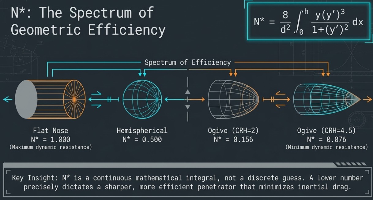
Nose factor \(N^*\) — Eqs. (2), (3a)–(3c)
\(N^*\) is defined by a surface integral over the nose profile. For standard geometries the integral has closed form:
| Nose type | \(\psi\) definition | \(N^*\) formula | Range |
|---|---|---|---|
| Flat | — | \(1.0\) | — |
| Ogive | CRH \(= R/d\) | \(\dfrac{1}{3\psi} - \dfrac{1}{24\psi^2}\) | \(0 < N^* < 0.5\) |
| Conical | \(H/d\) | \(\dfrac{1}{1 + 4\psi^2}\) | \(0 < N^* < 1.0\) |
| Spherical | \(r/d\) | \(1 - \dfrac{1}{8\psi^2}\) | \(0.5 < N^* < 1.0\) |
\(N^*\) is a continuous function of geometry, not a discrete lookup. A lower value means a sharper, more penetration-efficient nose: flat nose \(N^* = 1.0\) , hemispherical \(N^* = 0.5\) , ogive CRH=2 \(N^* = 0.156\) , ogive CRH=4.5 \(N^* = 0.076\) .
Nose height \(H/d\)
| Nose type | \(H/d\) |
|---|---|
| Flat | \(0\) |
| Ogive | \(\sqrt{\psi - 1/4}\) |
| Conical | \(\psi\) |
| Spherical | \(\psi - \sqrt{\psi^2 - 1/4}\) |
Crater depth parameter \(k\) — Eq. (25)
The crater–tunnel transition depth is the sum of the Prandtl plastic slip depth for a flat punch (\(0.707d\) ) and the nose height \(H\) :
| Nose | \(\psi\) | \(k\) |
|---|---|---|
| Flat | — | 0.707 |
| Hemispherical | 0.5 | 1.207 |
| Ogive CRH=2 | 2 | 2.030 |
| Ogive CRH=3 | 3 | 2.365 |
| Ogive CRH=4.5 | 4.5 | 2.769 |
| Output | Symbol | Unit |
|---|---|---|
| Nose shape factor | \(N^*\) | — |
| Dimensionless crater depth | \(k\) | — |
Node 2 — Target Resistance
Purpose. Compute the empirical constant \(S\) that scales the uniaxial compressive strength \(f_c\) to the effective resistance under dynamic triaxial confinement. \(S\) cannot be derived analytically; it is back-calculated from penetration tests and then fitted as a function of \(f_c\) .
| Input | Symbol | Unit |
|---|---|---|
| Unconfined compressive strength | \(f_c\) | MPa |
Two correlations are provided (\(f_c\) in MPa for both):
Original — Forrestal et al. (1994), Eq. (12):
Simplified — Li & Chen (2003), Eq. (21):
The simplified form makes \(I\) proportional to \(f_c^{-1/2}\) , aligning with the \(f_c\) dependence in NDRC, Hughes and Chang and enabling direct comparison. For \(f_c > 30\,\text{MPa}\) the two correlations are practically equivalent.
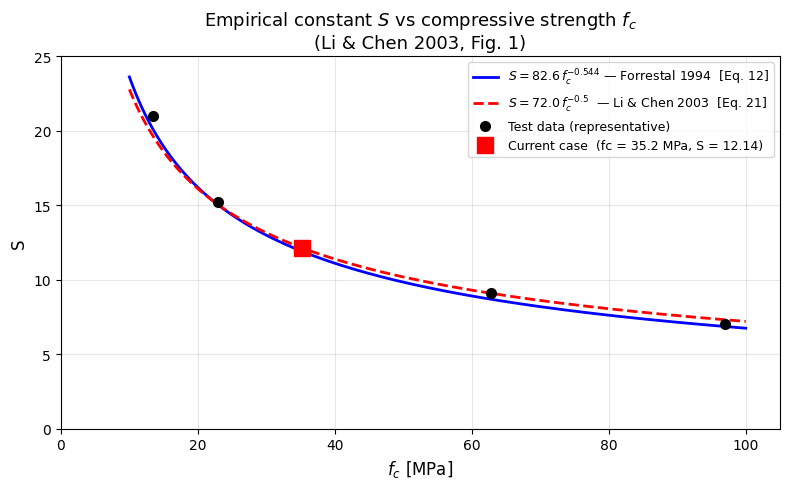
| \(f_c\) (MPa) | \(S_{\text{orig}}\) | \(S_{\text{simpl}}\) | \(S\) (paper) |
|---|---|---|---|
| 13.5 | 21.0 | 19.6 | 21 |
| 23 | 15.5 | 15.0 | 15.2 |
| 35.2 | 12.7 | 12.1 | 12 |
| 62.8 | 9.2 | 9.1 | — |
| 97 | 7.2 | 7.3 | 7 |
For shot 14 (\(f_c = 35.2\,\text{MPa}\) , \(S = 12\) from Table 2), both correlations agree to within 0.7 units.
| Output | Symbol | Unit |
|---|---|---|
| Target resistance constant | \(S\) | — |
Node 3 — Dimensionless Numbers
Purpose. Compute the two numbers that govern the penetration depth.
| Input | Symbol | Unit |
|---|---|---|
| Projectile mass | \(M\) | kg |
| Impact velocity | \(V_0\) | m/s |
| Shank diameter | \(d\) | m |
| Compressive strength | \(f_c\) | Pa |
| Concrete density | \(\rho_c\) | kg/m³ |
| Nose factor (Node 1) | \(N^*\) | — |
| Target resistance (Node 2) | \(S\) | — |
Intermediate quantities
Impact factor (Eq. 5):
Mass ratio (Eq. 6):
Johnson damage number (Eq. 7, informational):
\(\Phi_J\) depends only on velocity and target — not on the projectile. It classifies impact severity independently of the launcher.
Operational numbers
\(I\) is the ratio of projectile kinetic energy to the concrete’s effective absorption capacity (resistance under confinement, scaled by \(S\) , over volume \(d^3\) ).
\(N\) combines relative projectile mass and nose sharpness. A heavy, sharp projectile has large \(N\) and penetrates more for equal \(I\) .
| Output | Symbol | Unit |
|---|---|---|
| Impact function | \(I\) | — |
| Geometry function | \(N\) | — |
| (Intermediate) impact factor | \(I^*\) | — |
| (Intermediate) mass ratio | \(\lambda\) | — |
| (Intermediate) Johnson number | \(\Phi_J\) | — |
Node 4 — Regime Selection
Purpose. Determine whether the projectile stops inside the crater or advances into the tunnel.
| Input | Symbol | Unit |
|---|---|---|
| Impact function (Node 3) | \(I\) | — |
| Crater depth (Node 1) | \(k\) | — |
The projectile exits the crater zone with residual velocity \(V_1 > 0\) if and only if \(I > \pi k / 4\) :
| Output | — |
|---|---|
| Regime: shallow or deep | |
| Threshold value \(\pi k / 4\) |
Node 5a — Shallow Penetration — Eq. (15a)
Condition: \(X/d \leq k\) (projectile stops within the crater zone)
Derived from the energy balance \(X^2 = MV_0^2/c\) with the crater force constant \(c\) from the continuity condition at \(x = kd\) :
Consistency checks. At the regime boundary \(I = \pi k/4\) : the formula gives \(X/d = k\) , matching the deep formula below. For \(N \gg 1\) : reduces to Eq. (16a) of the paper. For \(N \gg 1\) and \(I/N \ll 1\) : reduces to \(X/d = \sqrt{4kI/\pi}\) , Eq. (17a).
Note on shallow correction. For \(X/d < 0.5\) the formula systematically overestimates (paper Fig. 11). The empirical correction Eq. (27) — \(\left(X/d\right)_{\text{corr}} = 1.628\,(X/d)^{2.789}\) — is available in the notebook as an opt-in flag. It is off by default: the correction was fitted on flat-nosed, low-energy data where scatter is large, and its applicability to other nose types is uncertain.
| Output | Symbol | Unit |
|---|---|---|
| Dimensionless penetration depth | \(X/d\) | — |
Node 5b — Deep Penetration — Eq. (15b)
Condition: \(X/d > k\) (projectile traverses the crater and bores a tunnel)
Derived by integrating the equation of motion \(MV\,dV/dx = -(\pi d^2/4)(Sf_c + N^*\rho_c V^2)\) from \(x = kd\) to \(x = X\) , then non-dimensionalising through \(I\) and \(N\) :
Penetration depth grows logarithmically with \(I\) at fixed \(N\) — not linearly. Each additional unit of velocity buys progressively less depth.
Consistency checks. At the regime boundary \(I = \pi k/4\) : \(\ln(1) = 0\) , giving \(X/d = k\) — exact continuity with Eq. (15a). For \(N \gg 1\) : reduces to Eq. (16b). For \(N \gg 1\) and \(I/N \ll 1\) : reduces to \(X/d = k/2 + 2I/\pi\) , Eq. (17b).
| Output | Symbol | Unit |
|---|---|---|
| Dimensionless penetration depth | \(X/d\) | — |
Node 6 — Dimensional Output
Purpose. Convert \(X/d\) to physical depth and summarise all intermediate values.
Report also: regime, \(I\) , \(N\) , \(k\) , \(S\) , \(I^*\) , \(\lambda\) , \(\Phi_J\) , and the semi-infinite check (\(3X\) minimum target thickness).
Numerical Verification — Shot 14
Forrestal et al. (1994), Table 3. Ogive CRH=2, \(f_c = 35.2\,\text{MPa}\) .
Input
| Quantity | Value |
|---|---|
| \(M\) | 0.906 kg |
| \(d\) | 0.0269 m |
| \(V_0\) | 277 m/s |
| Nose | ogive, \(\psi = 2\) |
| \(f_c\) | 35.2 MPa |
| \(\rho_c\) | 2370 kg/m³ |
Node 1
Note: paper Tables 2–4 use \(k = 2\) (empirical value from Forrestal 1994). The tool uses \(k = 2.030\) from Eq. (25). For this verification, \(k = 2\) is used to reproduce the paper tables.
Node 2
Node 3
Node 4
Node 5b
Paper Table 2, shot 14: \(X/d_{\text{anal}} = 6.21\) ✓ — \(X/d_{\text{test}} = 6.43\) — \(X/d_{\text{NDRC}} = 5.11\)
Node 6
Test: 173 mm. Error: 3.4%. Semi-infinite check: \(3X = 502\,\text{mm}\) minimum target thickness.
Figures
For fixed \(N\) , \(X/d\) grows logarithmically with \(I\) in the deep regime. The shallow-to-deep transition (knee of each curve) shifts with \(k\) and \(N\) . The current case is marked in red.
For fixed \(I\) , deeper penetration results from a heavier, sharper projectile (large \(N\) ). The sensitivity to \(N\) decreases as \(I/N \to 0\) — for shot 14 (\(I/N = 0.067\) ) geometry contributes marginally and \(X/d\) is driven almost entirely by \(I\) .
How to Use the Notebook
The Python notebook implements the full pipeline (Nodes 0–6) and runs directly on Google Colab. No installation required: numpy and matplotlib are preinstalled.
Modify only the INPUT PARAMETERS cell. Parameters:
| Parameter | Variable | Unit | Note |
|---|---|---|---|
| Projectile mass | M | kg | |
| Shank diameter | d | m | |
| Impact velocity | V0 | m/s | |
| Nose type | nose_type | — | "flat", "ogive", "conical", "spherical" |
| Nose parameter | psi | — | CRH for ogive, \(H/d\) for conical, \(r/d\) for spherical |
| Compressive strength | fc | Pa | e.g. 35.2e6 for 35.2 MPa |
| Concrete density | rho_c | kg/m³ | |
| \(S\) correlation | S_correlation | — | "simplified" (default) or "original" |
| Shallow correction | apply_shallow_correction | — | False (default); enable for \(X/d < 0.5\) |
Each node prints its full output — all intermediate values are visible.
Known limitations. The model requires: rigid (non-deformable) projectile — erosion becomes significant above ~800 m/s for hardened steel; semi-infinite target — rear boundary effects (scabbing, perforation) not modelled, verify thickness \(\geq 3X\) ; normal incidence — oblique impact not covered; unreinforced or lightly reinforced concrete (\(< 1.5\%\) per direction); aggregate size small relative to diameter (\(d/a > 5\) recommended, continuum assumption breaks down below \(d/a \approx 2\) ).
References
[1] Li QM, Chen XW (2003). Dimensionless formulae for penetration depth of concrete target impacted by a non-deformable projectile. Int. J. Impact Eng. 28, 93–116.
[2] Forrestal MJ, Altman BS, Cargile JD, Hanchak SJ (1994). An empirical equation for penetration depth of ogive-nose projectiles into concrete targets. Int. J. Impact Eng. 15(4), 395–405.
[3] Forrestal MJ, Luk VK (1988). Dynamic spherical cavity-expansion in a compressible elastic-plastic solid. ASME J. Appl. Mech. 55, 275–279.
[4] Sliter GE (1980). Assessment of empirical concrete impact formulas. ASCE J. Struct. Div. 106(ST5), 1023–1045.