Interactive Calculator
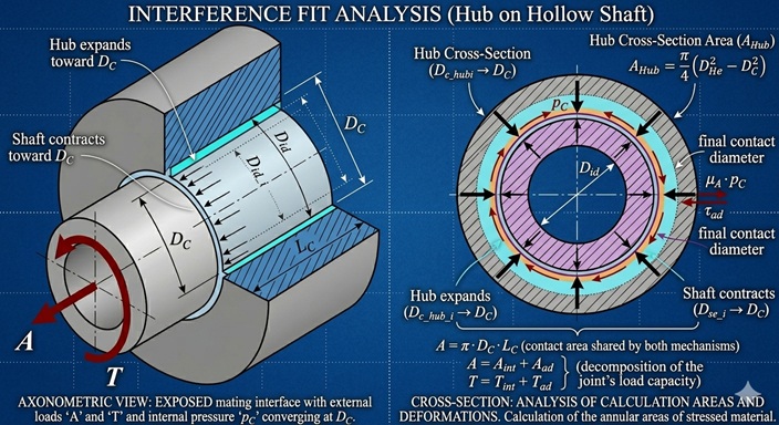
A shaft–hub connection transmits torque through two parallel mechanisms: friction from the interference fit pressure, and bonding shear from an adhesive film applied at the contact interface. The classical approach sizes the hub by experience or iteration — pick a wall thickness, check Tresca, adjust. Croccolo, De Agostinis & Vincenzi (2012) showed that for a given shaft diameter and material pair, an analytically optimal hub ratio \(Q_H = D_C / D_{He}\) exists that maximizes the torque-to-mass ratio of the joint. They derived a closed-form expression for this optimum that depends on only two dimensionless parameters: \(\phi\) (density–geometry ratio) and \(\chi\) (adhesive–strength ratio).
This tool implements that optimization as a six-step calculation pipeline. The pipeline takes shaft and hub materials, geometry, friction coefficient, and adhesive strength as input, and returns the optimal hub ratio \(Q_{H\_opt}\) , the corresponding Tresca-limited contact pressure \(p_C\) , the coupling geometry (\(D_C\) , \(D_{He}\) , \(L_C\) , \(Z\) ), and the design merit \(\text{DFLS}_T\) in kN·m/kg. A Python notebook ready to run on Google Colab is provided alongside the derivation, so every intermediate value can be verified.
Quick Example
A steel 39NiCrMo3 shaft must transmit a static torque \(T = 1.0\) kN·m through a hub in aluminum EN-AW6082. The allowable shaft shear stress is \(\tau_{allow} = 350\) MPa, the friction coefficient is \(\mu_T = 0.4\) . Three progressively more efficient designs:
| Scenario (a) | Scenario (b) | Scenario (c) | |
|---|---|---|---|
| Configuration | Solid shaft, no adhesive | Hollow shaft, no adhesive | Hollow shaft + adhesive |
| \(Q_S\) | 0 | 0.7 | 0.7 |
| \(\tau_{ad}\) (MPa) | 0 | 0 | 10 |
Design merit: (a) 5.92 kN·m/kg → (b) 8.86 kN·m/kg → (c) 11.68 kN·m/kg
Going from a solid shaft to a hollow shaft with adhesive nearly doubles the torque-to-mass ratio. The pipeline quantifies exactly how much each design choice contributes.
Pipeline summary:
| Step | Operation | Key output |
|---|---|---|
| 1 | Shaft sizing from torsion | \(D_C\) |
| 2 | Normalizing parameters | \(\phi\) , \(\chi\) |
| 3 | Optimal hub ratio | \(Q_{H\_opt}\) |
| 4 | Tresca pressure limit | \(p_C\) |
| 5 | Joint geometry | \(L_C\) , \(D_{He}\) , \(Z\) |
| 6 | Design merit | mass, \(\text{DFLS}_T\) |
Pipeline Overview
The pipeline is fully closed-form — no iteration, no solver. Each step feeds the next with explicit formulas. The normalizing parameters \(\phi\) and \(\chi\) collapse all material and geometry combinations into a two-parameter family, so the same pipeline applies to any shaft–hub pair from magnesium to steel.
Step 1 — Shaft Sizing
Purpose. Determine the minimum coupling diameter \(D_C\) from the required torque and shaft material.
| Symbol | Description | Unit |
|---|---|---|
| \(T\) | Required torque | N·mm |
| \(\tau_{allow}\) | Allowable shaft shear stress | MPa |
| \(Q_S = D_{Si}/D_C\) | Shaft bore ratio (0 for solid shaft) | — |
From the torsional section modulus of a hollow circular cross-section:
Note: the paper’s Eq. (30) uses \((1 - Q_S^3)\) rather than the exact \((1 - Q_S^4)\) . For \(Q_S = 0\) both forms are identical. For \(Q_S = 0.7\) the difference is about 5% on \(D_C\) . This tool follows the paper’s convention for verification consistency.
| Symbol | Description | Unit |
|---|---|---|
| \(D_C\) | Coupling diameter | mm |
Step 2 — Normalizing Parameters
Purpose. Reduce the material and geometry inputs to two dimensionless groups that fully characterize the optimization problem.
| Symbol | Description | Unit |
|---|---|---|
| \(Q_S\) | Shaft bore ratio | — |
| \(\rho_S\) , \(\rho_H\) | Shaft and hub densities | kg/mm³ |
| \(\tau_{ad}\) | Adhesive shear strength | MPa |
| \(S_{y\_H}\) | Hub yield strength | MPa |
\(\phi\) measures the relative weight contribution of the shaft: high \(\phi\) means the shaft dominates the joint mass (heavy material, solid section), pushing the optimum toward thinner hubs. \(\chi\) measures how much “free” shear capacity the adhesive adds relative to the hub’s yield limit. Two problems with identical \((\phi, \chi, \mu)\) have identical \(Q_{H\_opt}\) regardless of the actual materials and diameters.
| Symbol | Description | Unit |
|---|---|---|
| \(\phi\) | Density–geometry parameter | — |
| \(\chi\) | Adhesive–strength parameter | — |
Step 3 — Optimal Hub Ratio
Purpose. Find the hub aspect ratio \(Q_H\) that maximizes the torque-to-mass ratio \(\text{DFLS}_T\) .
| Symbol | Description | Unit |
|---|---|---|
| \(\phi\) , \(\chi\) | Normalizing parameters | — |
| \(\mu\) | Friction coefficient | — |
Without adhesive (\(\chi = 0\) ), Eq. (25) of the paper:
With adhesive (\(\chi > 0\) ), Eq. (29) of the paper:
For \(\chi = 0\) the second form reduces identically to the first. For \(\phi \to 1\) the denominator vanishes but the limit is finite: \(Q_{H\_opt} \to 1/\sqrt{2} \approx 0.707\) .
The approximation \(\mu^2 \ll 1/(1-Q_H^2)^2\) is used in deriving both forms. The paper’s Table 2 confirms the error on \(Q_{H\_opt}\) stays below 5% for all practical \((\phi, \mu)\) combinations.
| Symbol | Description | Unit |
|---|---|---|
| \(Q_{H\_opt}\) | Optimal hub ratio | — |
Step 4 — Tresca Pressure Limit
Purpose. Compute the maximum contact pressure the hub can sustain at the optimal \(Q_H\) before yielding at the inner surface.
| Symbol | Description | Unit |
|---|---|---|
| \(Q_{H\_opt}\) | Optimal hub ratio | — |
| \(\mu\) | Friction coefficient | — |
| \(\tau_{ad}\) | Adhesive shear strength | MPa |
| \(S_{y\_H}\) | Hub yield strength | MPa |
The Tresca criterion at the hub bore, combined with friction and adhesive shear on the interface, gives a quadratic in \(p_C\) . Defining:
For \(\tau_{ad} = 0\) this simplifies to:
| Symbol | Description | Unit |
|---|---|---|
| \(p_C\) | Tresca-limited contact pressure | MPa |
Step 5 — Joint Geometry
Purpose. Size the coupling length, hub outer diameter, and required interference.
| Symbol | Description | Unit |
|---|---|---|
| \(T\) | Required torque | N·mm |
| \(D_C\) | Coupling diameter | mm |
| \(p_C\) | Contact pressure | MPa |
| \(\mu\) , \(\tau_{ad}\) | Friction coefficient, adhesive strength | —, MPa |
| \(Q_{H\_opt}\) , \(Q_S\) | Hub and shaft bore ratios | — |
| \(E_S\) , \(\nu_S\) , \(E_H\) , \(\nu_H\) | Elastic constants | MPa, — |
Coupling length from torque equilibrium, Eq. (6):
Hub outer diameter:
Required diametral interference from Lamé compatibility, Eq. (3):
| Symbol | Description | Unit |
|---|---|---|
| \(L_C\) | Coupling length | mm |
| \(D_{He}\) | Hub outer diameter | mm |
| \(Z\) | Required diametral interference | mm |
Step 6 — Design Merit
Purpose. Compute the joint mass and the design function for lightweight structures.
| Symbol | Description | Unit |
|---|---|---|
| \(D_C\) , \(D_{Si}\) , \(D_{He}\) | Coupling, bore, and hub diameters | mm |
| \(L_C\) | Coupling length | mm |
| \(\rho_S\) , \(\rho_H\) | Shaft and hub densities | kg/mm³ |
| \(T\) | Required torque | N·m |
\(\text{DFLS}_T\) does not depend on \(D_C\) : at fixed materials and ratios, a joint transmits torque with the same mass efficiency regardless of absolute scale. This is a structural property of the torque case (where \(T \propto D_C^2\) and \(m \propto D_C^2\) ).
| Symbol | Description | Unit |
|---|---|---|
| \(m\) | Joint mass | kg |
| \(\text{DFLS}_T\) | Torque-to-mass ratio | N·m/kg |
Numerical Case — Croccolo et al. (2012), §4.1
Input
| Property | Shaft (39NiCrMo3 Steel) | Hub (EN-AW6082 Al) |
|---|---|---|
| \(\rho\) (kg/mm³) | \(7.87 \times 10^{-6}\) | \(2.75 \times 10^{-6}\) |
| \(E\) (MPa) | 207 000 | 69 000 |
| \(\nu\) | 0.29 | 0.33 |
| \(S_y\) (MPa) | — | 304 |
\(T = 1000\) N·m, \(\tau_{allow} = 350\) MPa, \(\mu_T = 0.4\) .
Scenario (a) — Solid shaft, no adhesive
\(Q_S = 0\) , \(\tau_{ad} = 0\) MPa.
Step 1. \(D_C = (16 \times 10^6 / (\pi \cdot 350 \cdot 1))^{1/3} = 24.4\) mm. Paper rounds to 25 mm.
Step 2. \(\phi = (1 - 0) \cdot 7.87/2.75 = 2.862\) . \(\chi = 0\) .
Step 3. \(Q_{H\_opt} = \sqrt{(1 - \sqrt{2.862})/(1 - 2.862)} = 0.610\) . Paper: 0.61. ✓
Step 4. \(p_C = 304 / (2\sqrt{1/(1-0.61^2)^2 + 0.16}) = 92.6\) MPa. Paper: 93 MPa. ✓
Step 5. \(L_C = 2 \times 10^6 / (0.4 \cdot 93 \cdot \pi \cdot 25^2) = 27.4\) mm. Paper: 28 mm. ✓. \(D_{He} = 25/0.61 = 41.0\) mm. \(Z = 0.093\) mm.
Step 6. \(m = 168.9\) g. \(\text{DFLS}_T = 1000/0.169 = 5920\) N·m/kg ≈ 5.92 kN·m/kg. Paper: 5.9. ✓
Scenario (b) — Hollow shaft, no adhesive
\(Q_S = 0.7\) , \(\tau_{ad} = 0\) MPa.
Step 1. \(D_C = (16 \times 10^6 / (\pi \cdot 350 \cdot 0.657))^{1/3} = 28.1\) mm. Paper: 28 mm. ✓
Step 2. \(\phi = (1 - 0.49) \cdot 2.862 = 1.460\) . \(\chi = 0\) .
Step 3. \(Q_{H\_opt} = \sqrt{(1 - \sqrt{1.46})/(1 - 1.46)} = 0.673\) . Paper: 0.67. ✓
Step 4. \(p_C = 81.2\) MPa. Paper: 82 MPa. ✓
Step 5. \(L_C = 24.8\) mm. Paper: 25 mm. ✓. \(D_{He} = 41.6\) mm. \(Z = 0.128\) mm.
Step 6. \(m = 112.9\) g. \(\text{DFLS}_T = \) 8.86 kN·m/kg. Paper: 8.9. ✓
Scenario (c) — Hollow shaft + adhesive
\(Q_S = 0.7\) , \(\tau_{ad} = 10\) MPa.
Step 2. \(\phi = 1.460\) (same as b). \(\chi = 2 \cdot 10 / 304 = 0.0658\) .
Step 3. \(Q_{H\_opt} = 0.725\) . Paper: 0.73. ✓
Step 4. \(p_C = 69.8\) MPa. Paper: 70 MPa. ✓
Step 5. \(L_C = 21.3\) mm. Paper: 21 mm. ✓. \(D_{He} = 38.7\) mm. \(Z = 0.126\) mm.
Step 6. \(m = 85.6\) g. \(\text{DFLS}_T = \) 11.68 kN·m/kg. Paper: 11.7. ✓
Summary
| (a) Solid, dry | (b) Hollow, dry | (c) Hollow + adhesive | |
|---|---|---|---|
| \(\phi\) | 2.862 | 1.460 | 1.460 |
| \(\chi\) | 0 | 0 | 0.066 |
| \(Q_{H\_opt}\) | 0.610 | 0.673 | 0.725 |
| \(p_C\) (MPa) | 92.6 | 81.2 | 69.8 |
| \(D_{He}\) (mm) | 41.0 | 41.6 | 38.6 |
| \(L_C\) (mm) | 27.4 | 24.8 | 21.3 |
| mass (g) | 168.9 | 112.9 | 85.6 |
| \(\text{DFLS}_T\) (kN·m/kg) | 5.92 | 8.86 | 11.68 |
All values within 3% of the paper. The 4.2% discrepancy on \(p_C\) for scenario (c) is structural: the paper applies the simplified Tresca form without \(\mu^2\) , while the calculator uses the full quadratic. \(\text{DFLS}_T\) is unaffected (0.2% deviation).
DFLS vs Hub Ratio
The chart in the calculator shows \(\text{DFLS}_T\) as a function of \(Q_H\) for the three canonical scenarios. Each curve rises from zero (infinitely thick hub), peaks at the analytic optimum \(Q_{H\_opt}\) , and falls back to zero (infinitely thin hub, Tresca forces \(p_C \to 0\) ). The adhesive shifts the peak rightward (thinner hub is optimal) and upward (higher merit). The three faded reference curves remain visible as context while the cyan curve tracks the current input configuration.
How to Use the Notebook
The Python notebook implements the full six-step pipeline and runs directly on Google Colab with no installation required (numpy and matplotlib are preinstalled).
Modify only the cell marked ✏️ Input. The parameters are:
| Parameter | Symbol | Unit | Note |
|---|---|---|---|
| Shaft density | rho_S | kg/mm³ | e.g. \(7.87 \times 10^{-6}\) for steel |
| Shaft Young’s modulus | E_S | MPa | |
| Shaft Poisson’s ratio | nu_S | — | |
| Hub density | rho_H | kg/mm³ | |
| Hub Young’s modulus | E_H | MPa | |
| Hub Poisson’s ratio | nu_H | — | |
| Hub yield strength | Sy_H | MPa | Tresca-governing |
| Shaft bore ratio | Q_S | — | 0 for solid shaft; ≤ 0.8 |
| Required torque | T | N·m | Static |
| Allowable shaft shear | tau_allow | MPa | |
| Friction coefficient | mu | — | Typically 0.1–0.4 |
| Adhesive shear strength | tau_ad | MPa | 0 for dry joint |
Known limitations. The model assumes plane stress, axisymmetric geometry, and linear-elastic isotropic materials (\(\sigma_{VM} < \sigma_y\) must hold). Hub yielding at the inner surface governs (Tresca criterion). The approximation \(\mu^2 \ll 1/(1-Q_H^2)^2\) is embedded in the \(Q_{H\_opt}\) formulas (error < 5% per Table 2 of the paper). Static torque only — no fatigue, no dynamic loads. Shaft buckling for hollow shafts (\(Q_S > 0.8\) ) is not checked. The paper’s Eq. (30) uses \((1 - Q_S^3)\) for the torsional section modulus instead of the exact \((1 - Q_S^4)\) .
References
[1] Croccolo, D., De Agostinis, M. & Vincenzi, N. (2012). Design and optimization of shaft–hub hybrid joints for lightweight structures. International Journal of Mechanical Sciences, 56(1), 77–85.
[2] Croccolo, D. & Vincenzi, N. (2009). A generalized theory for shaft–hub couplings. Proc. IMechE Part C: J. Mechanical Engineering Science, 223, 2231–2239.